
In aviation meteorology articles we often focus on the big problems: thunderstorms, heavy fog, low ceilings, and icing, all of which are responsible for the majority of weather-related aviation accidents. But even the most seemingly benign weather sometimes gets the best of IFR-rated pilots. In this Wx Smarts article we’ll revisit one such situation that took place in March 2020.
The airplane in question was a Piper PA-28R Arrow that was returning to Ohio after a long trip to Oklahoma. At the controls was a 42-year old businessman, a native of Ohio, who was working in the banking and real estate field. He held multi-engine and airline transport ratings and had logged 1500 hours of flight time. He was also a qualified flight instructor in single-engine aircraft.
On this night he flew alone. It was a nighttime flight under an IFR flight plan, flown at 11,000 feet, and all went normally. Approaching Cincinnati at 0212Z the Cherokee began a routine descent, with the destination being the municipal airport at Batavia, Ohio (KI69). The pilot requested an RNAV approach. Light winds at Batavia were 230 degrees at eight knots, and the ceiling was 600 feet with a visibility of 7 miles—no problem for an instrument-rated pilot. Radar showed scattered patchy showers moving out of the area that seemed to present no issues there either.
The pilot flew to the initial approach fix (IAF) at 3000 feet. At that point the controller saw that the airplane began an unexpected left-hand turn. The pilot claimed an autopilot malfunction and began a long right-hand turn back to the IAF. Approaching the next waypoint three minutes later, the airplane began a sharp right-hand turn. The controller asked the pilot if there were problems, and he replied that he was flying manually and encountering heavy turbulence and heavy downdrafts.
About 30 seconds later the airplane began a sharp descending left-hand turn, spiraling into the ground. The controller issued a low altitude alert, but the airplane was already in trouble. The Piper crashed in a wooded area a few miles north of Pleasant Plain, Ohio, claiming the life of the pilot.
Assembling the Puzzle Pieces
Within days, investigators began sifting through the wreckage. No problems could be found. Forensic analysis showed that the airplane was in good working order before the crash. However the with widespread IMC and showers in the area, the weather conditions were clearly suspect. A check of Leidos Flight Services showed that there was no contact on record with a flight weather briefer.
Digging further through the weather information, investigators found that the G-AIRMET products identified an area of low-level wind shear (LLWS) centered on the crash area, covering much of southern Ohio and southeast Indiana. Some thundershowers were in the region but no SIGMETs were in effect.
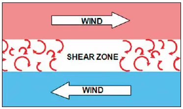
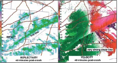
High-resolution NEXRAD radar data (this page, lower left) showed a highly sheared environment in the low levels, with bands of low-velocity and high-velocity air on the velocity image on the right. The difference between the bands was only about 20 knots. But it’s not the velocity that counts, it’s the shear, with shear being the difference in velocity per unit of linear distance. Indeed the very fact that we see distinct bands instead of a gradual transition from dark green to light green is a red flag that high amounts of shear are concentrated along the contact zone between the two areas. This region is known as the shear zone. (next page, top right)
The bands likely formed due to some sort of complex wave process, such as the development of gravity waves or Kelvin-Helmholtz instability. Whatever the case, the track of the aircraft (black line) showed that the airplane suffered its two major control upsets along the fringes of these bands.
An interesting feature on the radar images is the granular, patchy look of the velocities in the northern high-velocity band. This was even more ragged and mottled on lower-elevation radar tilts below 2500 feet. This indicates a highly turbulent layer, likely to be either due to wave breaking processes in the sheared environment or from convective downdrafts associated with the passing showers raining down into the sampling volume. Both are possible suspects in this case.
About half an hour after the crash, newer NEXRAD imagery (this page, lower right) showed a striking example of a shear line extending northeast to southwest across the region. It was drifting southeast at about 20 mph across the area. This marked either a front or a convergence line, and backtracking it to the accident time it was located near the first course deviation.
So clearly the atmosphere was highly unsettled and producing significant localized turbulence. The big mystery in this case is whether the unfortunate pilot ran into extreme amounts of shear, or whether the pilot was not up to the task of keeping the plane in the air in the challenging conditions with no visual references. Though we will never know the answer, the NTSB cited spatial disorientation and the loss of airplane control in darkness as the official accident cause.
Wind Shear Takeaways
Regardless of the ultimate cause, the lesson learned is that the effects of wind shear should not be underestimated. Quite often when we talk about severe turbulence the focus is on thunderstorms, mountain waves, and jet-stream clear-air turbulence. But as we’ve just seen, relatively benign weather patterns can produce the type of shear and turbulence that can knock small planes around.
 It should be reiterated that the G-AIRMET product warned about low-level wind shear, and this would have probably caught the pilot’s attention in a weather briefing. The Cincinnati aviation forecast desk just hours before the crash also mentioned the low-level wind shear problem in internal discussions. This setup was due to very strong shear between the surface and the atmosphere a couple of thousand feet off the ground, as shown on the Wilmington, Ohio, sounding (next page).
While you likely don’t have all of these tools at your disposal, the graphics we’ve shown are meant to illustrate what aviation forecasters are seeing when they confront these problems. Some clues you can use as a pilot that hint at wind shear problems are the presence of: (1) wind gusts on the METAR, (2) fronts and inversions in the local area accompanied by strong jet stream activity, (3) banded low cloud structures, (4) convective weather of any type, and of course (5) pilot reports reporting shear and low-level turbulence. Strong air mass modification—in particular intense heating of a relatively cool air mass from below—also amplifies mechanical turbulence and can manifest itself as wind shear. And of course don’t forget the presence of a “WS” group in the TAF.
 A Closer Look
Let’s take a closer look at wind shear and break things down a little further. Meteorologists divide wind shear into two basic types: horizontal shear and vertical shear. Horizontal shear describes wind differences on a horizontal plane. The strong differences along a cold front are a good example. The microburst that downed Delta 191 at DFW 40 years ago was defined by its strong horizontal shear, which caused significant airspeed losses as the airplane moved horizontally through the circulation.
Near Denver International Airport, researchers have used special Doppler radars to show horizontal shear along large summertime boundaries breaking off into eddies, which are then stretched vertically by thunderstorm updrafts, producing tall landspouts. Chances are you may know an airline pilot who’s flown into Denver who has stories about these long, pencil-like tornadoes.
There’s also vertical shear. This is an expression of differences in the wind vector between altitudes. In an unstable atmosphere, strong vertical shear is especially effective at generating turbulence. Severe weather forecasters also closely monitor low-level vertical shear because it directly enhances tornadic storms. Because of this, there is a severe weather chart found on many Internet sites called “0-1 km SRH (storm relative helicity).” You can actually use this chart to get a ballpark idea where low-level shear problems are. Values of over 200 indicate significant LLWS problems.
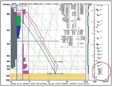 In the example above that caused the crash in Ohio, highly dynamic horizontal and vertical shear processes were taking place. We visualized the horizontal shear on the radar scans, and we saw the vertical shear on the sounding diagram. Both of these combined with deadly results.
And of course these shear circulations are not steady-state processes. They represent the dispersion of energy from larger to smaller scales. Shear breaks up into eddies that pilots and their passengers feel as turbulence. These eddies break down further all the way to molecular scales, where we are finally left with friction and heat. This is encapsulated in the saying by mathematician Lewis Fry Richardson: “Big whirls have little whirls that feed on their velocity, and little whirls have lesser whirls and so on to viscosity.”
Thunderstorms, Microbursts
Of course thunderstorm shear deserves special mention. The crash of Delta Flight 191 was a watershed moment in aviation meteorology where the danger of thunderstorm wind circulations at airports was recognized. Although severe turbulence is one of those hazards, the loss of airspeed at critical phases of flight is a key characteristic of thunderstorm shear.
The microburst produces the most deadly type of thunderstorm shear, as it represents a compact circulation of intense winds with a scale of only a few miles or less. This small scale means that aircraft undergo rapid variations in airspeed in only a matter of seconds. The microburst should not be thought of as a distinct phenomenon, but part of a spectrum of different intensities and scales of downdrafts and downbursts.
Because of this, all thunderstorms have some degree of potential to produce hazardous winds. The famous downburst that hit Andrews Air Force Base in 1983 shortly after Ronald Reagan’s plane landed, produced winds of 150 mph. This and the Delta Flight 191 storm both occurred in early August when no organized severe weather was expected.
The smaller, compact structure of a microburst is usually associated with very strong instability along with dry air aloft, mostly above 15,000 feet MSL. Strong microbursts often produce downdraft speeds of greater than 3000 fpm in their core. If your airplane cannot achieve this kind of climb rate, well, you probably know what comes next.
Downdrafts, downbursts, and microbursts can all manifest themselves visually. For example, you might see curl in a downdraft rain shaft that can form into a “rain foot” where the rain shaft spreads out laterally. You could also see dust clouds and even debris lofted along the leading edge of the downdraft. Gustnadoes can also form, which are tornado-like whirls close to the ground where the shear zone has wrapped up and is stretched vertically. These are identifiable as fast-moving plumes of dust measuring tens to hundreds of feet wide.
Although the effect of downbursts and microbursts above the surface is often not visible, the leading edge often contains a long horizontal vortex, very similar to the roll cloud associated with mountain waves. Severe turbulence can be expected anywhere near this zone.
When you’re in the traffic pattern and thunderstorms are nearby, it pays to keep an eye out for all of these visual features, as they can suddenly appear in about a minute and can quickly engulf the airfield. Once the visual indications disappear and wind speeds die down, which usually follows in about 10 or 20 minutes, the airfield is probably once again safe.
Airborne weather radar is of very limited use for avoiding wind shear and microburst hazards. Radars with turbulence detection however are an exception, since this uses information from the velocity channel. The reflectivity (intensity) display, however, is too coarse for airborne radar to pick up outflow and microburst structure, because the radars are specifically tuned to detect water and ice.
NEXRAD radars are extremely sensitive and often detect thunderstorm outflow due to the dust, debris, insects, and other detritus that are lofted into the air and scatter as the storm passes. A meteorologist at a workstation will be able to track outflow boundaries, downbursts, and microbursts without much difficulty, but in the cockpit there is too much latency and workload for tools like ADS-B to be of much help.
Your view out the cockpit window, observations from the tower, and reports from ASOS sites are far more useful tools for knowing what’s going on. And of course if things look too questionable, don’t hesitate to wait the storm out. Remember that every pilot listed as a fatality in the NTSB records due to weather was almost certainly confident they had the situation under control until, well, they didn’t.
Tim Vasquez was an Air Force forecaster and briefed countless B-1B, C-130, and C-5 pilots on wind shear hazards. You can catch some of his videos on YouTube by searching for “Forecast Lab.”.


