
Stability and instability are topics that come up a lot in aviation meteorology. Perhaps it’s been a little too long since ground school and you need a refresher. You’ve come to the right place. Physics concepts like humidity, pressure, density, and stability can sometimes be difficult to remember, and the topics are about as dry as it gets. But these things do play into the safety of your flight, and understanding them will make you a sharper pilot. So let’s begin.
Some Basic Concepts
When we consider a column of air through the troposphere, the layer of air about 20,000 to 50,000 feet deep, we find that the temperature always decreases within this layer as a whole. Smaller layers embedded within this column, including those in contact with the surface, often show different characteristics. These layers may be isothermal, showing no temperature change with height, or may increase in temperature with height, creating an inversion. The layer above the troposphere, the stratosphere, always shows an isothermal layer or an inversion, and we use this to help find the top of the troposphere.
Time to introduce a new term: the lapse rate. The authoritative Glossary of Meteorology by the American Meteorological Society (available free online!) defines it as a change of a variable with height. Typically this is temperature. We often discuss the lapse rate of the standard atmosphere, which is 3.6 Fahrenheit degrees per thousand feet. Lapse rates often vary through the column, so when we discuss them it’s important to explain which altitudes we’re discussing.
In meteorology we sometimes define a lapse rate by the change of temperature using pressure coordinates. The 700-500 mb or 700-500 hPa lapse rate has been a staple of severe weather forecasting for decades and is sometimes referred to in forecasting discussions. This is simply the temperature difference between the two levels. This in turn is used in instability indexes such as the Vertical Totals and Total Totals Index.
A lapse rate that shows the normal, expected cooling with height is positive lapse rate. When it shows rapid cooling with height, we refer to it as a “steep lapse rate” or “high lapse rate,” and this usually suggests weather, turbulence, gusty winds, or storms. When it shows warming with height, it is a negative lapse rate, but in meteorology we just call it an “inversion.”
Adiabatic Cooling
Here’s where things get a little complicated. When we take a given volume of air and force it to ascend or descend, its temperature changes. This is due to the ideal gas law, which is not about the airport with the best price on 100LL but rather relates temperature, pressure, and volume of a gas to one another. Take the example of a weather balloon at an altitude of 20,000 feet that is suddenly forced to 10,000 feet, and we disregard heat lost or absorbed from the outside. The balloon encounters denser air with more pressure, which forces the volume to contract, pushing the molecules in the balloon closer together and increasing the temperature within the system. The temperature goes up.
Fortunately this temperature change is very predictable and can be described by a change known as the dry adiabatic lapse rate (DALR). This lapse rate is about 5.4 Fahrenheit degrees per 1000 feet, but varies according to the pressure, the altitude, and the actual temperature.
Sometimes latent heat is being released while a parcel of air ascends. This process occurs all the time in clouds. When this happens, the rate of cooling with height diminishes due to the added heat, and the temperature changes according to the moist adiabatic lapse rate. A ballpark figure on this is about 2.7 Fahrenheit degrees per 1000 feet. As we can see, that latent heat really adds a lot of warmth to the parcel, and this is the main mechanism by which hurricanes get so powerful.
Stability and Instability
Static instability is associated with a steep lapse rate. We can simplify this to a layer that is very cold on top and very warm at the bottom, or “cold over warm.” Stability is the opposite: it is a layer which is relatively isothermal or warms with height. We can just refer to it as “warm over cold.”
We can best understand the concept of static stability using an imaginary balloon. This balloon starts out at, let’s say 5000 feet MSL at a temperature of 12 degrees C. Both the air inside the balloon and the air outside are at equilibrium, and both have a temperature of 12 degrees C.
In the case of statically stable air, we apply a force pushing the balloon down to 4500 feet MSL. Note that the temperature increases by an arbitrary amount to 14 degrees C due to adiabatic warming. But since stable air is a “warm over cold” setup, we find cooler air down below. Our balloon is warmer than the surrounding air, so it resists our attempt to push it downward and returns to its original level where it seeks equilibrium. If it overshoots the original level, it becomes cooler than the surrounding air and seeks its original level.
But in statically unstable air, when we apply this same force, we encounter surrounding air that is much warmer, since this is a “cold over warm” setup. Our balloon becomes much cooler than the surrounding air. The causes an increasing downward acceleration. Our balloon sinks even faster, going down like the proverbial lead balloon. Likewise, if we force the balloon upward instead, it will keep accelerating upward, because the atmosphere cools faster than the balloon does.
You might expect the threatening, slightly orange colors in the illustration to be in the “unstable atmosphere” example. But a stable atmosphere is hazy and traps pollutants, and they accumulate since they can’t disperse into the free atmosphere. On the other hand, the unstable atmosphere promotes mixing through deep layers, and tends to have unusually clear visibility.
Those of you in the central United States might be familiar with muggy, hazy conditions on a high-risk storm day, and wonder where the clear visibilities are. Ceiling and visibility actually show an improving trend as heating takes place. However air masses in this region are often “capped” by a mid-tropospheric inversion that traps moisture and haze until later in the day. Higher in the atmosphere, we do find layers with steep lapse rates and high instability, and good visibility is found at these altitudes.
Stability Layers
 You have to recognize that the atmosphere often contains multiple stable and unstable layers that combine in different ways. Things would be incredibly simple if the atmosphere was a simple stable column or an unstable one. Forecasters would just check a box and clock out for the day.
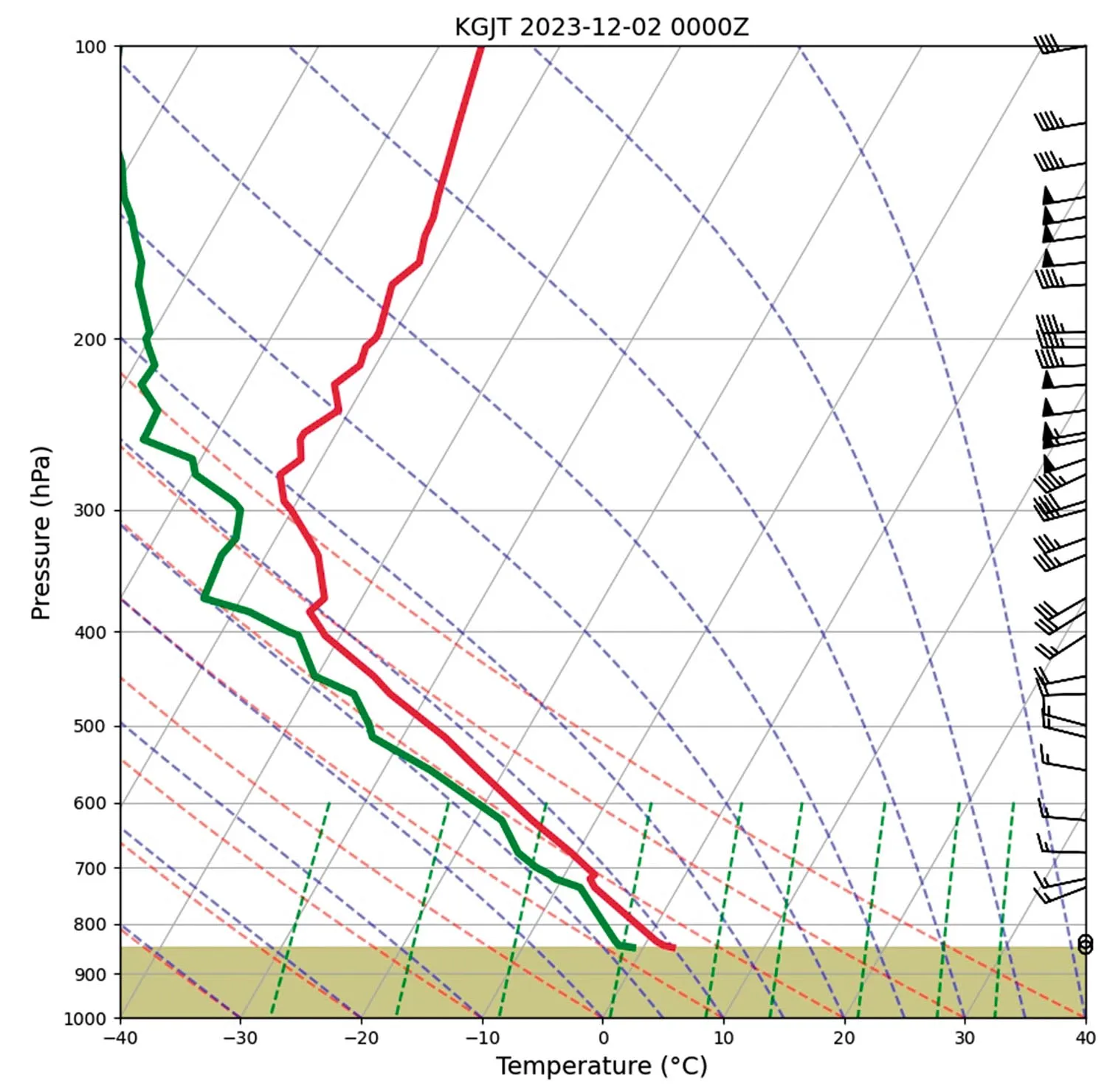
To unravel this ball of yarn, forecasters refer to a thermodynamic diagram. There are many types: the tephigram, the emagram, the Stüve diagram, and even the pastagram! Many of these were developed in the late 19th century as physicists worked out the behavior of gases. But the Skew-T is the diagram that has come into most common use. It was created in 1947 and used extensively by U.S. Air Force meteorologists. It worked its way into civilian use by the 1960s and is now recognized worldwide.
By plotting the temperature at different altitudes, we get a graph known as a sounding. Of course it’s not just temperature that’s important but also the profile of moisture with height, so we also plot the dew point. If you want to learn a bit more about soundings, we covered it in the January 2022 issue. By looking at the slope of the sounding through different layers, we can immediately identify the stability. The more the temperature line leans to the left with height within a given layer, the greater the lapse rate and the greater the instability in that layer.
There are many different weather processes that affect the lapse rate. Large scale dynamic lift, through the action of mid-level weather disturbances, helps destabilize the atmosphere and steepen lapse rates. Differential advection, such as when cool upper-level flow arrives from Canada and contrasts with tropical low-level flow, can also destabilize the atmosphere. One of the tasks of forecasters is to understand these processes that are taking place and how they will affect the stability profiles in different layers.
Mechanical Turbulence
Turbulence that develops due to interaction with terrain is often referred to as “mechanical turbulence.” Why do we experience it on some days with windy conditions but not on other days? The lapse rate is the key.
Very strong heating due to abundant sunlight or the passage of a fresh, cold air mass over warm terrain both contribute to a “cold over warm” setup. In both cases, heat is transferred into the air mass from the bottom up, resulting in kinetic motion, acceleration of air parcels, and the development of turbulent eddies.
This is one reason why the region just behind fast-moving cold fronts are prime locations for low-level turbulence, especially in the presence of solar heating as clouds begin breaking up. On the other hand, the region ahead of warm fronts experience the opposite—a stable “warm over cold” setup that doesn’t favor turbulence.
But always be wary of vertical shear, particularly with low-level jets in the Central U.S. that sometimes cross these warm fronts. Though surface layers are not favored for turbulence, altitudes near the low-level jet at roughly 1000 to 4000 feet often have different lapse-rate profiles and can generate some light to moderate chop.
Clear Air Turbulence (CAT)
Now we get into clear air turbulence. Again, stability and instability are important because these processes modulate how vertical oscillations are transformed over space and time.
Classic clear air turbulence develops when there is instability in the middle or upper troposphere. When steep lapse rates develop, air is more easily able to rise and fall when acted on by outside forces, such as by winds that are out of balance. Vertical motions are more likely to amplify over time, eventually resulting in overturning and wave-breaking action that produces turbulent structures through disintegration of large-scale flow.
Vertical wind shear, in other words, the change of the wind vector with height (usually through the change in wind velocity) profoundly increases the risk of CAT. This was recognized as far back as the 1950s, and helped form some of the earliest turbulence forecasting rules. When shear is present in a layer, it departs from smooth laminar flow and the layer is more likely to develop that which can grow into larger structures conducive to CAT.
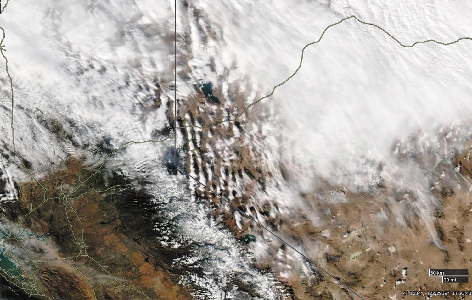
Interestingly, mountain wave turbulence such as that seen near the Sierras, Rockies, and Appalachians favors a stable layer at mountain altitude. The barrier effect produces an oscillating vertical wave, which is maintained in the relatively stratified air downstream from the mountains as the atmosphere tries to re-establish equilibrium. These waves can sometimes be seen as spectacular standing lenticular altocumulus clouds. (“Standing” refers to their lack of movement.)
However when unstable layers exist above or below this altitude, the mountain wave oscillations can be transferred downward or upward, forming turbulent structures such as rotors. This is most likely to occur when relatively warm terrain exists downwind from the mountains, which destabilizes a layer (remember “cold over warm”) below the stratified mountain wave layer. Severe turbulence might occur in the lower levels, such as that which was partly involved in the loss of a United 737 at Colorado Springs in 1991. It may also occur within or above the stratified mountain wave layer, as with the downing of a British Airways 707 near Mt. Fuji in 1966.
Getting Sharper
Hopefully we’ve given you some new topics to think about. It’s essential to start looking at some Skew-T diagrams if you want to delve into the world of stability. A good place to start is the Storm Prediction Center website (www.spc.noaa.gov); just click on the Forecast Tools menu item and you’ll find the latest data. Give it a try, learn to read the chart, and compare it to what you see out the airplane window. I guarantee you will find the experience highly educational and somewhat illuminating.
Tim Vasquez was an aviation forecaster in the U.S. Air Force and trained all the incoming meteorologists at Dyess AFB and at the Korea Theater Forecast Unit at Yongsan Garrison. He now brings his training to IFR, Weatherwise, and YouTube.


